As a grad student, just entering the world of object detection i found it quite helpful, that there are a lot of resources especially blog posts, made easy to quickly digest complex concepts and ideas. If you type in related search phrases you will find some splendid results on how to calculate the mean Average Precision (mAP) on the first page. The explanation of the basic components is mostly in a very easy and straightforward manner, but sometimes just did not explain the calculation of the mAP correctly. This confused me a lot which is why i came to write this blog post of my findings.
This post assumes you have already grasped a basic understanding about the steps up until calculating the mAP and is aimed to aid you in having a comprehensive information overview and tries to offer further explanation and intuition.
Why mean Average Precision
When training an object detection model you want to quantify and compare different models and tell which model performs better than the other. Not only is the correct classification but also the correct localization decisive for the quality of your model. A go to metric is the mean Average Precision (mAP).
Training the model, will occur with a training data set. To verify the quality of your model, it will then be applied to a test or validation data set, which is independent of the training data. The mAP is calculated over the result of your model’s prediction on your validation data set.
Intersection over Union (IoU)
Whether a detection is correct or not solely dependents on the model’s predicted bounding box of an object and its overlap with the original bounding box of the object in the image (ground truth). This is also called Intersection over Union (IoU). Padilla et al., 2020[1] explained the IoU with a very simple and easy to understand image (see image 1, green = ground truth, red = bounding box).
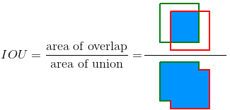
The result is a value between 0 and 1. The higher the value, the higher the overlap which in turn interprets as a better prediction. In general we could define any threshhold which fits our own definition as correct prediction. For better understanding, just imagine we set our threshhold to 0.5 meaning if our prediction overlaps 50% with the ground truth then it is a correct detection.
The IoU is object specific and the sole criteria, whether a detection of an object was correct or not (see Everingham et. al. 2010, p.11[2]). Say you have a prediction box for object A but the ground truth is actually object B. Therefore the IoU is non existent for the predicted object A, even though there exists a ground truth bounding box underneath.
Confusion Matrix – TP, FP, FN
To estimate our performance we can then calculate the confusion matrix’ metrics, based on the IoU threshhold.
True Positive (TP): We get an IOU > threshhold.
- This means, that we predicted a bounding box which has an overlap with the ground truth higher than the set threshhold.
False Positive (FP): We get an IOU < threshhold.
- Our model predicted a bounding box, which does not overlap well enough with the ground truth.
- OR it predicted a good positioned bounding box but the underlying true class is another one. In this case the IoU is non existent because there is no overlap of the predicted object with the true object (some would call this a misclassification).
- If an object has been detected multiple times, only the prediction with the highest confidence (not IoU) is counted as a TP, the other predictions will be counted as FP (see Everingham et. al. 2010, p.12 [2] ).
False Negative (FN): A ground truth not detected although the image actually contains the object.
True Negative (TN): Is not relevant since this only tells you the correctly non detection of bounding boxes.
- For example if we don’t predict a bounding box in a free space which also has no objects and no ground truth, this would be a TN. Since we are only interested in the correct detections, this metric is not relevant for us.
Precision and Recall can be calculated from the given metrics like so:
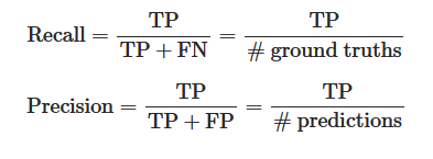
A high precision indicates, that a lot of predictions made are correct (low FP). While high recall indicates, that we actually found most of the objects (low FN). We can visualize the relationship between precision and recall in a precision recall curve.
Precision Recall Curve
I highly recommend and refer to Padilla et al., 2020[1] ‘s git repository where he illustrated the calculation on a comprehensive example. The following section only summarizes his work with some extended explanation. Interpolation is mentioned in the original paper of the Pascal VOC challenge ( see Everingham et. al. 2010, p.11[2]).
For each prediction we receive a confidence score and whether it’s a TP or a FP based on the IoU. Then we sort the result by descending order of confidence score and accumulate the TP and FP. Using the accumulated TP and FP we calculate the Precision and Recall for each prediction. This result can now be visualized as a Precision x Recall Curve.
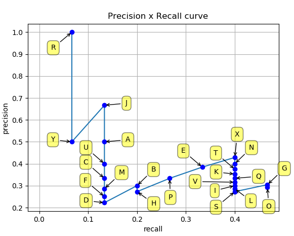
Naturally the curve will start with a high precision because most of the objects detected are correct (few FP), but a lot of objects are not detected at all (high FN) and therefore resulting in a low Recall value. As it proceeds the prediction list, a lot more objects are detected (decreases FN) which increasses the Recall value but also a lot of misdetections occur (increase of FP) which decreases the precision value.
A prediction model has a high quality if the Precision-Recall Curve stays high with increasing Recall values. This would indicate, that a lot of objects have been detected (low FN) while also not making many mistakes (low FP).
Average Precision
To indicate a model’s quality it would be best to have a single numeric value to compare different models instead having to compare every model by its curve. The Average Precision (AP) is meant to summarize the Precision-Recall Curve by averaging the precision across all recall values between 0 and 1. Efffectively it is the area under the Precision-Recall curve. Because the curve is a characterized by zick zack lines it is best to approximate the area using interpolation. At this point i would again like to refer to the already comprehensive work of Padilla et al., 2020[1] and also EL Aidouni, 2019[3] on how to interpolate the precision from the recall value given a Precision-Recall Curve. Take note that the interpolation is slightly different from challenge to challenge and can effect the resulting value.
For Pascal VOC challenge:
- Before 2010 a 11-Point Interpolation was used at Recall levels [0, 0.1, … , 1] (see Everingham et. al. 2010, p.11[2])
- after 2010 an all point interpolation is in use
For COCO challenge:
- A 101 point Interpolation is in use ( see cocodataset.org section 3, “recThrs”)
The mAP
Remember we only calculated the AP for one class. The average of APs across all classes would make the mean Average Precision (mAP).
It is important to note, that the mAP depends on the way you calculate the AP but more importantly it depends on the IoU threshold you defined to distinguish correct from uncorrect detections. Here again the different challenges define their calculation of the mAP differently.
For Pascal VOC they define an IoU threshold > 0.5 (see Everingham et. al. 2010, p.11[2]).
However for the COCO challenge the calculation for the primary mAP metric is the average mAP across all the IoU threshold between 0.5 and 0.95 with a step size of 0.05. Furthermore the mAP calculated at an IoU threshold of 0.5 was denoted as [email protected] and several other metrics with various specifications have been introduced ( see cocodataset.org section 2).
Sidenote:
Harshit Kumar’ blog post already mentions, that the way the Pascal VOC challenge calculates the mAP does not account for skewness of different IoU levels. A result with an IoU of 0.6 is equal to one with an IoU of 0.9. Let’s extend on his thought with an example. Below in Table 1 and Table 2 we see 4 detections.
| detection | IoU |
| 1 | 0.9 |
| 2 | 0.6 |
| 3 | 0.6 |
| 4 | 0.6 |
| detection | IoU |
| 1 | 0.9 |
| 2 | 0.9 |
| 3 | 0.9 |
| 4 | 0.6 |
For simplicity we assume that we only need to detect object A which is already ordered by confidence score. Let’s say there are only 4 objects to detect therefore no FN and the IoU threshold is 0.5 making every detection a TP. The mAP for both Table 1 and Table 2 would be the same (being 1), however the detection in table 2 is obviously the superior one because it has a better overall localisation indicated by the higher IoU scores.
So how do we consider this skewness? The COCO challenge resolved this issue by averaging the AP over multiple IoU thresholds, specifically from 0.5 to 0.95 with a 0.05 stepsize ( see cocodataset.org section 2, 1.). We can demonstrate this with our example and a simplified threshold of 0.5 and 0.75.
The AP for an IoU threshold of 0.5 is still 1 for both table 1 and 2. Let’s calculate the AP for an IoU threshold of 0.75:
| detection | IoU | TP | FP | acc TP | acc FP | Precision | Recall |
| 1 | 0.9 | 1 | 0 | 1 | 0 | 1/(1+0) = 1 | 1/(1+3) = 0.25 |
| 2 | 0.6 | 0 | 1 | 1 | 1 | 1/(1+1) = 0.5 | 1/(1+3) = 0.25 |
| 3 | 0.6 | 0 | 1 | 1 | 2 | 1/(1+2) = 0.33 | 1/(1+3) = 0.25 |
| 4 | 0.6 | 0 | 1 | 1 | 3 | 1/(1+3) = 0.25 | 1/(1+3) = 0.25 |
| detection | IoU | TP | FP | acc TP | acc FP | Precision | Recall |
| 1 | 0.9 | 1 | 0 | 1 | 0 | 1/(1+0) = 1 | 1/(1+1) = 0.5 |
| 2 | 0.9 | 1 | 0 | 2 | 0 | 2/(2+0) = 1 | 2/(2+1) = 0.66 |
| 3 | 0.9 | 1 | 0 | 3 | 0 | 3/(3+0) = 1 | 3/(3+1) = 0.75 |
| 4 | 0.6 | 0 | 1 | 1 | 1 | 3/(3+1) = 0.75 | 3/(3+1) = 0.75 |
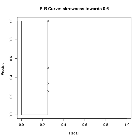
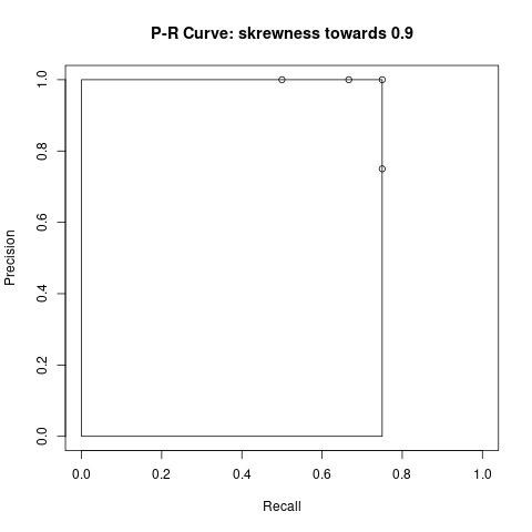
Take note that in Table 3 we have detection 2 to 4 with an IoU less than our threshold which results into FP. Additionally since these three objects were not detected, the FN count is 3. We always calculate precision and recall with the accumulated TP and FP values. The mAP is the area under the curve, indicated by the rectangle in image 4 and image 5.
Let’s calculate the mAP for the examples:
Example with skewness towards 0.6
- [email protected] = 1
- [email protected] = 0.25*1 = 0.25
- average mAP = (1 + 0.25) / 2 = 0.625
Example with skewness towards 0.9
- [email protected] = 1
- [email protected] = 0.75 * 1 = 0.75
- average mAP = (1 + 0.75) / 2 = 0.875
As to be expected now we observe a much higher mAP score for the detection example with overall higher IoU scores.
If you found this blog helpful or have any constructive criticism feel free to drop a comment 🙂
Further Readings
As mentioned, a comprehensive resource was this git repository from R. Padilla et. al. : https://github.com/rafaelpadilla/Object-Detection-Metrics . Although i was mising a bit of intuitive explanation and also the difference between all these challenges, which is why i came up with this blog post.
Manal El Aidouni provided a lot of intuition to the metrics and very nice visuals. A nitpick here: His section “Precision – recall and the confidence threshold” threw me off track and added a lot to my intial confusion. As i understand it’s more of a sidenote, than anything regarding the calculation of the mAP: https://manalelaidouni.github.io/manalelaidouni.github.io/Evaluating-Object-Detection-Models-Guide-to-Performance-Metrics.html
Harshit Kumar gives a much more dense overview than this post. It’s a very easy read if you are already involved with the topic.: https://kharshit.github.io/blog/2019/09/20/evaluation-metrics-for-object-detection-and-segmentation
Jonathan Hui’s blog post is also a nice write up, which i did not use as a resource though: https://jonathan-hui.medium.com/map-mean-average-precision-for-object-detection-45c121a31173
References
- Padilla, R., S. L. Netto, E. A. B. da Silva (2020). „A Survey on Performance Metrics for Object-Detection Algorithms“. In: 2020 International Conference on Systems, Signals and Image Processing (IWSSIP), p. 237–242. | git repository [↩][↩][↩][↩][↩]
- „The Pascal Visual Object Classes (VOC) Challenge“. In: International Journal of Computer Vision 88.2, S. 303–338. issn: 0920-5691, 1573-1405. doi:10.1007/s11263-009-0275-4. url: http://link.springer.com/10.1007/s11263-009-0275-4 (last visit 22. 11. 2020).[↩][↩][↩][↩][↩]
- EL Aidouni, Manal (5. Okt. 2019). Evaluating Object Detection Models: Guide to Performance Metrics. url: https://manalelaidouni.github.io/manalelaidouni.github.io/Evaluating-Object-Detection-Models-Guide-to-Performance-Metrics.html#average-precision (visitedam 05. 11. 2020). [↩]
Pingback: how to calculate map – Relevant Archive